
Generalized linear mixed model fit by maximum likelihood (Laplace
  Approximation) [glmerMod]
 Family: binomial  ( logit )
Formula: Dep.Var ~ After.New + Morph.Type + Before + Stress + Phoneme +
    (1 | Speaker)
   Data: td
Control: glmerControl(optCtrl = list(maxfun = 20000), optimizer = "bobyqa")

      AIC       BIC    logLik -2*log(L)  df.resid
     1114      1175      -545      1090      1177

Scaled residuals:
   Min     1Q Median     3Q    Max
-5.223 -0.488 -0.259  0.495 14.033

Random effects:
 Groups  Name        Variance Std.Dev.
 Speaker (Intercept) 0.796    0.892
Number of obs: 1189, groups:  Speaker, 66

Fixed effects:
            Estimate Std. Error z value Pr(>|z|)
(Intercept)   -0.277      0.207   -1.34  0.18034
After.New1     1.840      0.157   11.71  < 2e-16 ***
After.New2    -1.175      0.144   -8.14  4.1e-16 ***
Morph.Type1    0.426      0.140    3.05  0.00230 **
Morph.Type2   -1.892      0.213   -8.87  < 2e-16 ***
Before1       -0.575      0.202   -2.84  0.00447 **
Before2        0.526      0.193    2.72  0.00659 **
Before3        0.117      0.278    0.42  0.67370
Before4        0.731      0.190    3.85  0.00012 ***
Stress1       -0.799      0.137   -5.81  6.2e-09 ***
Phoneme1       0.287      0.128    2.25  0.02462 *
---
Signif. codes:  0 '***' 0.001 '**' 0.01 '*' 0.05 '.' 0.1 ' ' 1

Correlation of Fixed Effects:
            (Intr) Aft.N1 Aft.N2 Mrp.T1 Mrp.T2 Befor1 Befor2 Befor3 Befor4
After.New1   0.064
After.New2  -0.104 -0.430
Morph.Type1 -0.434  0.203 -0.114
Morph.Type2 -0.051 -0.221  0.178 -0.376
Before1     -0.296 -0.223  0.293  0.052  0.429
Before2     -0.164  0.191 -0.094 -0.110  0.247  0.029
Before3      0.150  0.018 -0.060  0.319 -0.515 -0.421 -0.477
Before4      0.250  0.304 -0.431 -0.202  0.051 -0.311 -0.090 -0.274
Stress1     -0.434 -0.432 -0.064  0.050  0.097  0.056  0.125 -0.094 -0.250
Phoneme1     0.459  0.149 -0.307 -0.137 -0.265 -0.543 -0.263  0.149  0.438
            Strss1
After.New1
After.New2
Morph.Type1
Morph.Type2
Before1
Before2
Before3
Before4
Stress1
Phoneme1 -0.107Mixed-Efects Logistic Regression Analysis: Part 3
Doing a mixed-effects logistic regression analysis suitable for comparing to a Goldvarb analysis. Part 3: Correlations, Interactions, & Collinearity
Before you proceed with this section, please make sure that you have your data loaded and modified based on the code here and that Dep.Var is re-coded such that Deletion is the second factor. Next, you set the global R options to employ sum contrast coding.
Correlations, Interactions, & Collinearity
Lets look again at the results of the most parsimonious analysis of the full data set.
Below the results for fixed effects is a table of the correlations of the fixed effects. This table is a good way to spot non-orthogonal effects you might not yet have caught (though you should have caught these effects if you thoroughly explored your data using summary statistics). Look at only the coefficients for the correlations of levels of different parameters. Generally any value over \(|0.3|\)1 should be investigated further. If you have any correlations over \(|0.7|\) you should be worried. In your table there is no correlation higher than \(|0.7|\), but there are a few over \(|0.3|\): After.New1*Before4 \(|0.304|\); After.New1*Stress1 \(|0.432|\); After.New2*Before4 \(|0.431|\); After.New2*Phoneme1 \(|0.307|\); Morph.Type1*Before3 \(|0.319|\); Morph.Type2*Before3 \(|0.515|\); Before1*Phoneme1 \(|0.543|\); and Before4*Phoneme1 \(|0.438|\). These correlations suggest it might be worthwhile to re-check the summary statistics, looking especially at the cross-tab of After.New and Before, After.New and Phoneme, Morph.Type and Before, Morph.Type and Phoneme, and Before and Phoneme.2
There are two other methods for testing for a relationship between your fixed effect predictors that relate to the kind of relationship your fixed effects predictors might have. The first is that the predictors have an interaction the other is that they are (multi-) collinear.
Interactions
An interaction arises when two independent fixed effects work together to predict the variation of the application value. For example, based on the Conditional Inference Tree analysis you know that it is not case that gender itself explains the social variation in Deletion vs. Realized (this is confirmed by the analysis of data from just young speakers, where Sex is not significant), nor is it that age explains the social variation (confirmed by the non-significance of both Age.Group and Center.Age in the full model). Instead, it seems that older men use Deletion more frequently than everyone else. This is an interaction. It is the combination of Age.Group and Sex that (potentially) best explains the social variation. You can test this in your model by creating an interaction group with these two fixed effect predictors. You do this by including the interaction term Sex*Age.Group in your analysis. To make things easier here you can simplify and again consider middle-age and older speakers together. You can also drop Phoneme as it is non-significant among both cohorts. When you include an interaction term, the individual components of the interaction will also be included as singular predictors.
# Create a simplified Age.Group.Simple column
td <- td %>% mutate(Age.Group.Simple = cut(YOB, breaks = c(-Inf, 1979, Inf),
                                  labels = c("Old/Middle", "Young")))

# Create a regression analysis with a Sex*Age.Group.Simple interaction group
td.glmer.sex.age.interaction <- glmer(Dep.Var ~ After.New + Morph.Type + Before + Stress + Sex*Age.Group.Simple + (1 | Speaker), data = td, family = "binomial", glmerControl(optCtrl = list(maxfun = 20000), optimizer = "bobyqa"))

summary(td.glmer.sex.age.interaction)
Generalized linear mixed model fit by maximum likelihood (Laplace
Approximation) [glmerMod]
Family: binomial ( logit )
Formula:
Dep.Var ~ After.New + Morph.Type + Before + Stress + Sex * Age.Group.Simple +
(1 | Speaker)
Data: td
Control: glmerControl(optCtrl = list(maxfun = 20000), optimizer = "bobyqa")
AIC BIC logLik -2*log(L) df.resid
1117 1188 -545 1089 1175
Scaled residuals:
Min 1Q Median 3Q Max
-4.305 -0.492 -0.266 0.492 14.222
Random effects:
Groups Name Variance Std.Dev.
Speaker (Intercept) 0.695 0.834
Number of obs: 1189, groups: Speaker, 66
Fixed effects:
Estimate Std. Error z value Pr(>|z|)
(Intercept) -0.4344 0.1831 -2.37 0.01767 *
After.New1 1.7895 0.1554 11.51 < 2e-16 ***
After.New2 -1.0791 0.1371 -7.87 3.6e-15 ***
Morph.Type1 0.4618 0.1385 3.34 0.00085 ***
Morph.Type2 -1.7712 0.2055 -8.62 < 2e-16 ***
Before1 -0.3258 0.1695 -1.92 0.05454 .
Before2 0.6685 0.1870 3.58 0.00035 ***
Before3 0.0159 0.2750 0.06 0.95385
Before4 0.5365 0.1696 3.16 0.00156 **
Stress1 -0.7696 0.1368 -5.63 1.8e-08 ***
Sex1 -0.2626 0.1359 -1.93 0.05322 .
Age.Group.Simple1 0.1281 0.1371 0.93 0.35011
Sex1:Age.Group.Simple1 -0.1750 0.1363 -1.28 0.19902
---
Signif. codes: 0 '***' 0.001 '**' 0.01 '*' 0.05 '.' 0.1 ' ' 1
Correlation matrix not shown by default, as p = 13 > 12.
Use print(x, correlation=TRUE)  or
vcov(x) if you need itAnova(td.glmer.sex.age.interaction)Analysis of Deviance Table (Type II Wald chisquare tests)
Response: Dep.Var
Chisq Df Pr(>Chisq)
After.New 144.21 2 < 2e-16 ***
Morph.Type 74.39 2 < 2e-16 ***
Before 36.42 4 2.4e-07 ***
Stress 31.67 1 1.8e-08 ***
Sex 3.71 1 0.054 .
Age.Group.Simple 0.71 1 0.399
Sex:Age.Group.Simple 1.65 1 0.199
---
Signif. codes: 0 '***' 0.001 '**' 0.01 '*' 0.05 '.' 0.1 ' ' 1What you can see from the summary(td.glmer.sex.age.interaction) and Anova(td.glmer.sex.age.interaction) results is that this interaction term is not significant and does not add explanatory value to the analysis. The negative polarity of the estimate coefficient of the interaction term Sex1:Age.Group.Simple1 indicates that when the level of Sex is Female (1) and Age.Group.Simple is Old/Middle (1) the overall probability decreases by \(-0.1750\). This coefficient represents the extra effect of both predictors working together. The \(p\)-value of \(0.19902\), however, indicates that this change is not statistically different from zero/no effect. In other words, even though we know older men use Deletion more frequently, the extra effect of combining age and sex does not emerge as significant when the influence of the linguistic predictors is considered. If you want to home in on the older/middle men in your results, you can reorder the Sex predictor. Using the fct_rev() function, which reverses the order of factors making the last “missing” factor first, is the easiest way to do this.
# Create a regression analysis with a Sex*Age.Group.Simple interaction group in which `Male` equals Sex1
td.glmer.sex.age.interaction <- glmer(Dep.Var ~ After.New + Morph.Type + Before + Stress + fct_rev(Sex)*Age.Group.Simple + (1 | Speaker), data = td, family = "binomial", glmerControl(optCtrl = list(maxfun = 20000), optimizer = "bobyqa"))

summary(td.glmer.sex.age.interaction)
Generalized linear mixed model fit by maximum likelihood (Laplace
Approximation) [glmerMod]
Family: binomial ( logit )
Formula: Dep.Var ~ After.New + Morph.Type + Before + Stress + fct_rev(Sex) *
Age.Group.Simple + (1 | Speaker)
Data: td
Control: glmerControl(optCtrl = list(maxfun = 20000), optimizer = "bobyqa")
AIC BIC logLik -2*log(L) df.resid
1117 1188 -545 1089 1175
Scaled residuals:
Min 1Q Median 3Q Max
-4.305 -0.492 -0.266 0.492 14.222
Random effects:
Groups Name Variance Std.Dev.
Speaker (Intercept) 0.695 0.834
Number of obs: 1189, groups: Speaker, 66
Fixed effects:
Estimate Std. Error z value Pr(>|z|)
(Intercept) -0.4344 0.1831 -2.37 0.01767 *
After.New1 1.7895 0.1554 11.51 < 2e-16 ***
After.New2 -1.0791 0.1371 -7.87 3.6e-15 ***
Morph.Type1 0.4618 0.1385 3.34 0.00085 ***
Morph.Type2 -1.7712 0.2055 -8.62 < 2e-16 ***
Before1 -0.3258 0.1695 -1.92 0.05454 .
Before2 0.6685 0.1870 3.58 0.00035 ***
Before3 0.0159 0.2750 0.06 0.95385
Before4 0.5365 0.1696 3.16 0.00156 **
Stress1 -0.7696 0.1368 -5.63 1.8e-08 ***
fct_rev(Sex)1 0.2626 0.1359 1.93 0.05323 .
Age.Group.Simple1 0.1281 0.1371 0.93 0.35011
fct_rev(Sex)1:Age.Group.Simple1 0.1750 0.1363 1.28 0.19902
---
Signif. codes: 0 '***' 0.001 '**' 0.01 '*' 0.05 '.' 0.1 ' ' 1
Correlation matrix not shown by default, as p = 13 > 12.
Use print(x, correlation=TRUE)  or
vcov(x) if you need itAnova(td.glmer.sex.age.interaction)Analysis of Deviance Table (Type II Wald chisquare tests)
Response: Dep.Var
Chisq Df Pr(>Chisq)
After.New 144.21 2 < 2e-16 ***
Morph.Type 74.39 2 < 2e-16 ***
Before 36.42 4 2.4e-07 ***
Stress 31.67 1 1.8e-08 ***
fct_rev(Sex) 3.71 1 0.054 .
Age.Group.Simple 0.71 1 0.399
fct_rev(Sex):Age.Group.Simple 1.65 1 0.199
---
Signif. codes: 0 '***' 0.001 '**' 0.01 '*' 0.05 '.' 0.1 ' ' 1You can see that the coefficient for the interaction term is identical, but with reverse polarity. It indicates that when Sex is Male and Age.Group.Simple is Old/Middle the extra effect is \(+0.1750\), but again, as you saw above, this difference is not significantly different from zero/no effect \(p = 0.19902\).
An alternative way to test this interaction is to create a four-way Sex:Age.Group.Simple interaction group and include it as a fixed effect. By doing this instead of testing for an extra effect caused by the interaction of these two variables, you are instead testing the difference in likelihood from the overall likelihood for each combination of age and sex, and determining whether this is significantly different from zero.
[1] "F:Old/Middle" "F:Young" "M:Old/Middle" "M:Young" The levels of the four-way interaction group are F:Old/Middle, F:Young, M:Old/Middle, and M:Young. If you recreate your glmer() analysis, you should find that the third level, M:Old/Middle, to have a positive coefficient (Deletion more likely than the mean), and the others to have a negative coefficient (Deletion less likely than the mean).
# Create a regression analysis with the Age.Simple:Sex interaction group
td.glmer.sex.age.interaction <- glmer(Dep.Var ~ After.New + Morph.Type + Before + Stress + Sex.Age.Group.Simple + (1 | Speaker), data = td, family = "binomial", glmerControl(optCtrl = list(maxfun = 20000), optimizer = "bobyqa"))

summary(td.glmer.sex.age.interaction)
Generalized linear mixed model fit by maximum likelihood (Laplace
Approximation) [glmerMod]
Family: binomial ( logit )
Formula:
Dep.Var ~ After.New + Morph.Type + Before + Stress + Sex.Age.Group.Simple +
(1 | Speaker)
Data: td
Control: glmerControl(optCtrl = list(maxfun = 20000), optimizer = "bobyqa")
AIC BIC logLik -2*log(L) df.resid
1117 1188 -545 1089 1175
Scaled residuals:
Min 1Q Median 3Q Max
-4.305 -0.492 -0.266 0.492 14.222
Random effects:
Groups Name Variance Std.Dev.
Speaker (Intercept) 0.695 0.834
Number of obs: 1189, groups: Speaker, 66
Fixed effects:
Estimate Std. Error z value Pr(>|z|)
(Intercept) -0.4344 0.1831 -2.37 0.01767 *
After.New1 1.7895 0.1554 11.51 < 2e-16 ***
After.New2 -1.0791 0.1371 -7.87 3.6e-15 ***
Morph.Type1 0.4618 0.1385 3.34 0.00085 ***
Morph.Type2 -1.7712 0.2055 -8.62 < 2e-16 ***
Before1 -0.3258 0.1695 -1.92 0.05454 .
Before2 0.6685 0.1870 3.58 0.00035 ***
Before3 0.0159 0.2750 0.06 0.95386
Before4 0.5365 0.1696 3.16 0.00156 **
Stress1 -0.7696 0.1368 -5.63 1.8e-08 ***
Sex.Age.Group.Simple1 -0.3095 0.2161 -1.43 0.15206
Sex.Age.Group.Simple2 -0.2158 0.2441 -0.88 0.37668
Sex.Age.Group.Simple3 0.5658 0.2557 2.21 0.02692 *
---
Signif. codes: 0 '***' 0.001 '**' 0.01 '*' 0.05 '.' 0.1 ' ' 1
Correlation matrix not shown by default, as p = 13 > 12.
Use print(x, correlation=TRUE)  or
vcov(x) if you need itAnova(td.glmer.sex.age.interaction)Analysis of Deviance Table (Type II Wald chisquare tests)
Response: Dep.Var
Chisq Df Pr(>Chisq)
After.New 144.21 2 < 2e-16 ***
Morph.Type 74.39 2 < 2e-16 ***
Before 36.42 4 2.4e-07 ***
Stress 31.67 1 1.8e-08 ***
Sex.Age.Group.Simple 5.62 3 0.13
---
Signif. codes: 0 '***' 0.001 '**' 0.01 '*' 0.05 '.' 0.1 ' ' 1By using this four-way interaction group you can see that the M:Older/Middle (Sex.Age.Group.Simple3) coefficient is negative, and it is significantly different from zero/no effect. To find the coefficient for the missing fourth value, re-create the analysis using fct_rev().
# Create a regression analysis with the reversed Age.Simple:Sex interaction group
td.glmer.sex.age.interaction <- glmer(Dep.Var ~ After.New + Morph.Type + Before + Stress + fct_rev(Sex.Age.Group.Simple) + (1 | Speaker), data = td, family = "binomial", glmerControl(optCtrl = list(maxfun = 20000), optimizer = "bobyqa"))

summary(td.glmer.sex.age.interaction)
Generalized linear mixed model fit by maximum likelihood (Laplace
Approximation) [glmerMod]
Family: binomial ( logit )
Formula:
Dep.Var ~ After.New + Morph.Type + Before + Stress + fct_rev(Sex.Age.Group.Simple) +
(1 | Speaker)
Data: td
Control: glmerControl(optCtrl = list(maxfun = 20000), optimizer = "bobyqa")
AIC BIC logLik -2*log(L) df.resid
1117 1188 -545 1089 1175
Scaled residuals:
Min 1Q Median 3Q Max
-4.305 -0.492 -0.266 0.492 14.222
Random effects:
Groups Name Variance Std.Dev.
Speaker (Intercept) 0.695 0.834
Number of obs: 1189, groups: Speaker, 66
Fixed effects:
Estimate Std. Error z value Pr(>|z|)
(Intercept) -0.4344 0.1831 -2.37 0.01767 *
After.New1 1.7895 0.1554 11.51 < 2e-16 ***
After.New2 -1.0791 0.1371 -7.87 3.6e-15 ***
Morph.Type1 0.4618 0.1385 3.34 0.00085 ***
Morph.Type2 -1.7712 0.2055 -8.62 < 2e-16 ***
Before1 -0.3258 0.1695 -1.92 0.05454 .
Before2 0.6685 0.1870 3.58 0.00035 ***
Before3 0.0159 0.2750 0.06 0.95386
Before4 0.5365 0.1696 3.16 0.00156 **
Stress1 -0.7696 0.1368 -5.63 1.8e-08 ***
fct_rev(Sex.Age.Group.Simple)1 -0.0405 0.2273 -0.18 0.85861
fct_rev(Sex.Age.Group.Simple)2 0.5658 0.2557 2.21 0.02692 *
fct_rev(Sex.Age.Group.Simple)3 -0.2158 0.2441 -0.88 0.37667
---
Signif. codes: 0 '***' 0.001 '**' 0.01 '*' 0.05 '.' 0.1 ' ' 1
Correlation matrix not shown by default, as p = 13 > 12.
Use print(x, correlation=TRUE)  or
vcov(x) if you need itAnova(td.glmer.sex.age.interaction)Analysis of Deviance Table (Type II Wald chisquare tests)
Response: Dep.Var
Chisq Df Pr(>Chisq)
After.New 144.21 2 < 2e-16 ***
Morph.Type 74.39 2 < 2e-16 ***
Before 36.42 4 2.4e-07 ***
Stress 31.67 1 1.8e-08 ***
fct_rev(Sex.Age.Group.Simple) 5.62 3 0.13
---
Signif. codes: 0 '***' 0.001 '**' 0.01 '*' 0.05 '.' 0.1 ' ' 1As with the other levels, Men:Young (fct_rev(Sex.Age.Group.Simple)1) is not significant. What you can conclude is that all women and young men are not significantly different from the overall probability (and by extension each other), but old/middle men are significantly different from the overall probability. Creating this four-way interaction group and including it as a fixed effect reveals this pattern in a way that including the interaction term Sex:Age.Simple does not. That being said, the results of the Anova() indicate that this predictor still does not add explanatory value to the analysis.
Collinearity
When fixed effects predictors are not independent we say they are (multi-) collinear. Collinearity and interactions are similar, but separate, phenomena.
Collinearity is the phenomenon whereby two or more predictor variables are highly correlated, such that the value/level of one can be predicted from the value/level of the other with a non-trivial degree of accuracy. Including both in an anlysis 1) violates the assumptions of the model; and 2) can actually result in diminished liklihood estimates for both predictors, masking real effects. As discussed before, in this Cape Breton data, Education, Job, and Age.Group are all collinear to various degrees. For example, if Job is Student, then the level of Education can be predicted (it will also be Student), and vice versa. For both, Age.Group can be predicted too (Young). These types of correlations are easy to see for social categories, but somewhat more difficult to tease out for linguistic categories. The first step is always a thorough cross tabulation of your independent variables. For a quick visual of cross tabulations you can employ a mosaic plot. Here is the code for creating a quick mosaic plot using ggplot2, which you likely already have installed if you’ve followed along with previous chapters.
# Install ggmosaic package
install.packages("ggmosaic")library(ggmosaic)
library(ggplot2)
# Create a quick mosaic plot of Phoneme and Before
ggplot(td)+
geom_mosaic(aes(product(Dep.Var, Before, Phoneme), fill = Dep.Var))+
theme_mosaic()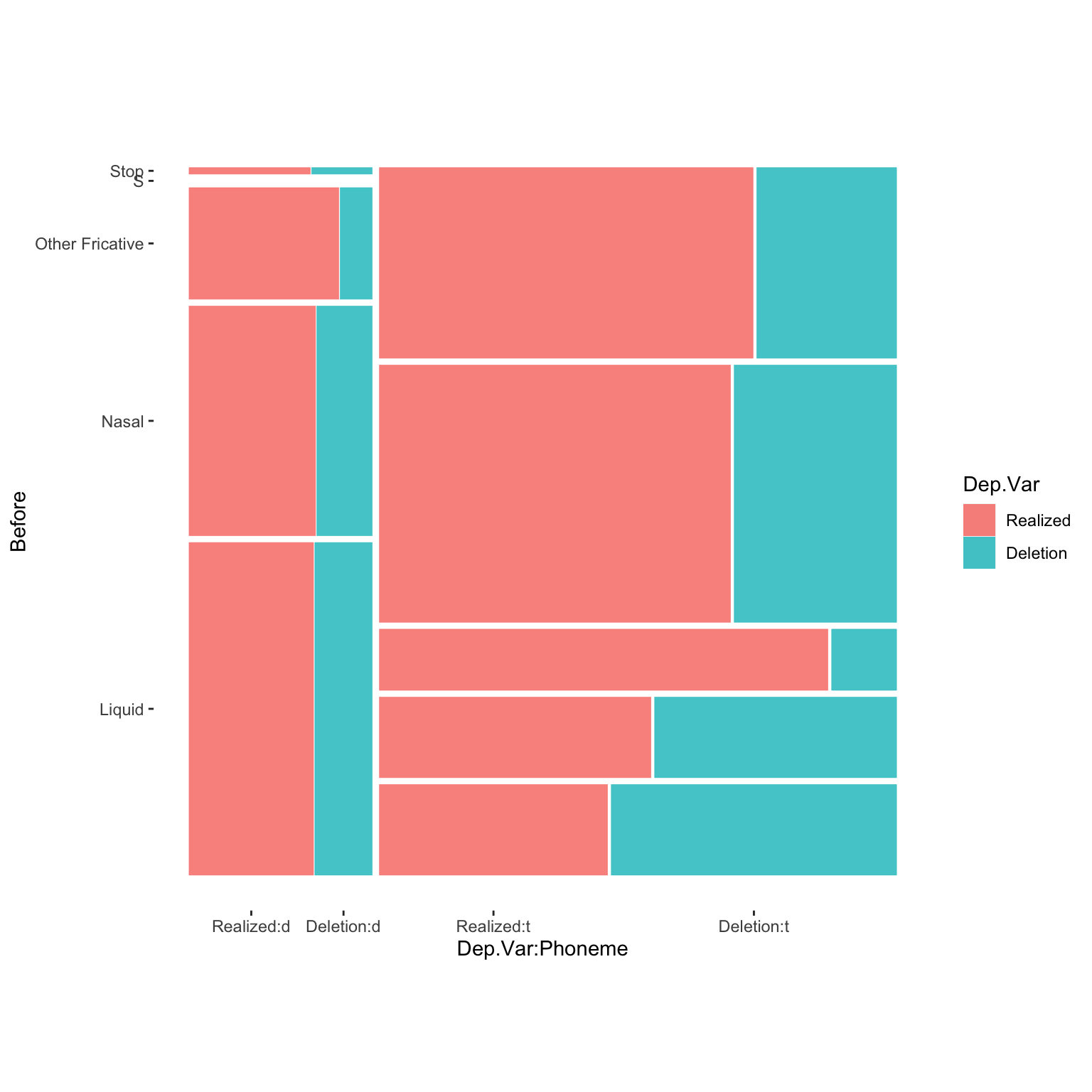
In a mosaic plot the size of the box for each combination of variables corresponds to the relative number of tokens of that combination. The first major observation from the mosaic plot is that there are no preceding /s/ tokens where the underlying phoneme is /d/, and there are remarkably few tokens in which /d/ is preceded by a non-nasal stop.3 This indicates that you shouldn’t include both of these predictors in your model, or complexify the model by creating a interaction group of Phoneme and Before. This is because you can predict some of the values of Phoneme and Before. For example, if a token is underlyingly world-final /d/, the preceding segment will not be /s/. Likewise, if the preceding segment is /s/, the underlying phoneme must be /t/.
Lets look at another mosaic plot.
# Create a quick mosaic plot of Phoneme and Before
ggplot(td)+
  geom_mosaic(aes(product(Dep.Var, Before, After.New), fill = Dep.Var))+
  theme_mosaic()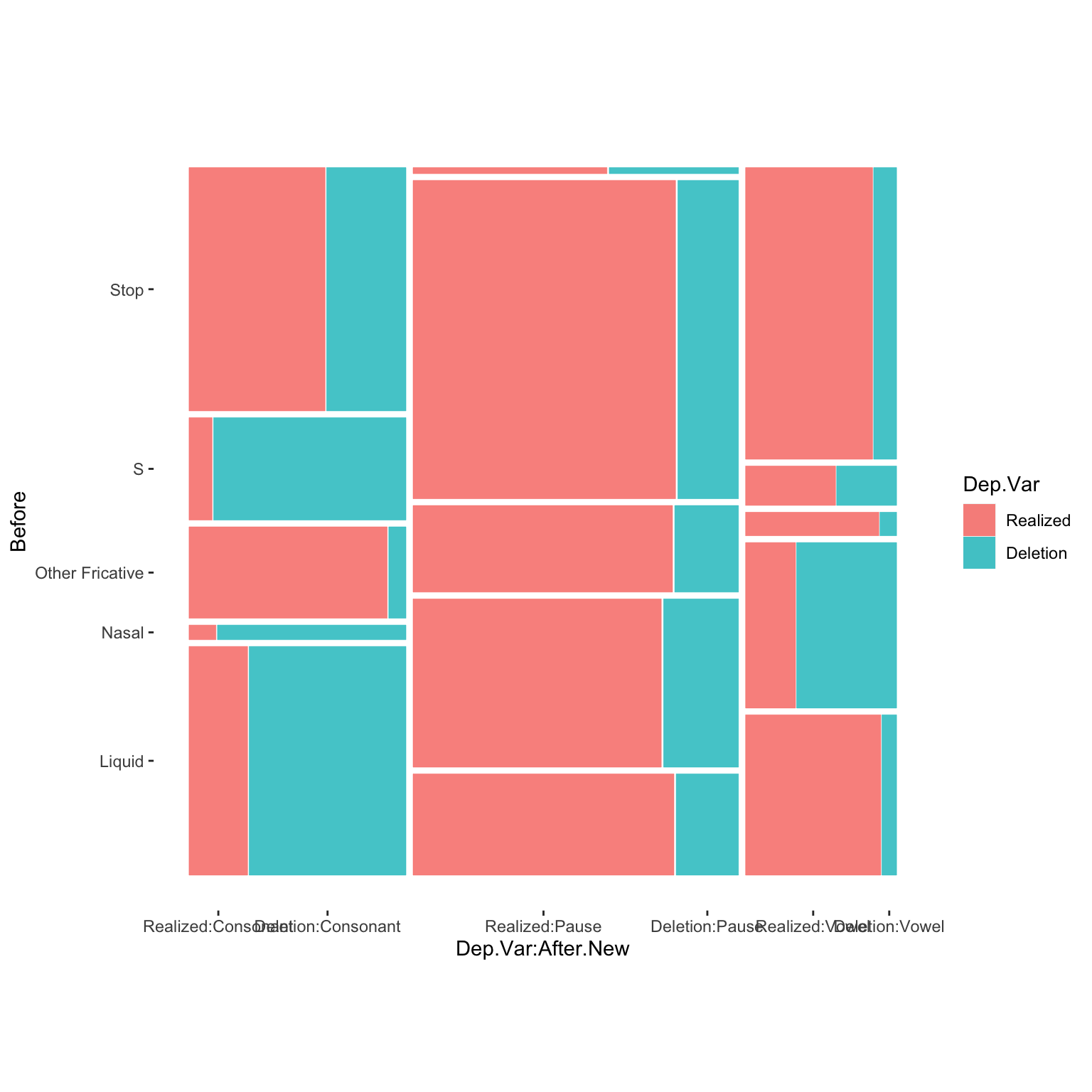
This plot is a little bit hard to read. To make the x-axis labels a little easier to read, you can use the binary version of Dep.Var. You’ll remember that 1 is Deletion and 0 is Realized.
# Create a quick mosaic plot of Phoneme and Before
ggplot(td)+
  geom_mosaic(aes(product(Dep.Var.Binary, Before, After.New), fill = Dep.Var.Binary))+
  theme_mosaic()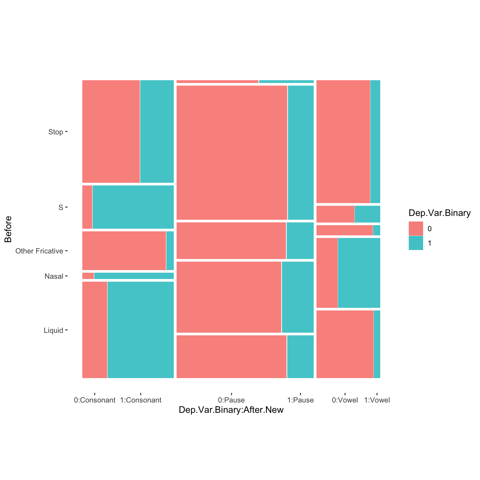
This mosaic plot show that there are very few tokens with a preceding Stop and a following Pause. Though no apparent collinearity is present, this mosaic plot does reveal some interesting potential interactions. The effect of preceding /s/, liquids, and nasals appears to be specific to pre-consonental contexts, and perhaps also pre-vowel contexts for nasals. This suggests further exploration of the data is warranted — perhaps by creating separate glmer() models for each following context, by complexifying your full model by creating a Before and After.New interaction group, or by simplifying your full model by collapsing these two categories into simpler grouped categories, e.g., Pre-Pause, Liquid-Consonant, Liquid-Vowel, Nasal-Consonant, Nasal-Vowel, S-Consonant, S-Vowel, Other-Consonant, Other-Vowel, or similar.
# Create a new model using insights from the mosaic plots
td<-td %>%
    mutate(Before.After = factor(paste(td$Before, td$After.New, sep =".")))%>%
    mutate(Before.After = recode_factor(Before.After,
                                 "Liquid.Pause" = "Pause",
                                 "Nasal.Pause" = "Pause",
                                 "Other Fricative.Pause" = "Pause",
                                 "S.Pause" = "Pause",
                                 "Stop.Pause" = "Pause",
                                 "Other Fricative.Consonant" = "Other.Consonant",
                                 "Stop.Consonant" = "Other.Consonant",
                                 "Other Fricative.Vowel"= "Other.Vowel",
                                 "Stop.Vowel" = "Other.Vowel"))


td.glmer.parsimonious.new <- glmer(Dep.Var ~ Before.After + Morph.Type + Stress + (1 | Speaker), data = td, family = "binomial", glmerControl(optCtrl = list(maxfun = 20000), optimizer = "bobyqa"))

# Compare fit of new parsimonious model with old parsimonious model
anova(td.glmer.parsimonious, td.glmer.parsimonious.new)
Data: td
Models:
td.glmer.parsimonious: Dep.Var ~ After.New + Morph.Type + Before + Stress + Phoneme + (1 | Speaker)
td.glmer.parsimonious.new: Dep.Var ~ Before.After + Morph.Type + Stress + (1 | Speaker)
npar AIC BIC logLik -2*log(L) Chisq Df Pr(>Chisq)
td.glmer.parsimonious 12 1114 1175 -545 1090
td.glmer.parsimonious.new 13 1087 1153 -531 1061 28.6 1 8.7e-08
td.glmer.parsimonious
td.glmer.parsimonious.new ***
---
Signif. codes: 0 '***' 0.001 '**' 0.01 '*' 0.05 '.' 0.1 ' ' 1The anova() function shows that td.glmer.parsimonious.new is a better fit model. In other words, it does a better job of predicting the variation in the data.
It is important, however, to point out that collinearity does not reduce the predictive power or reliability of the glmer() model as a whole — it only affects calculations regarding individual predictors. That is, a glmer() model with correlated predictors can indicate how well the entire bundle of predictors predicts the outcome variable, but it may not give valid results about any individual predictor, or about which predictors are redundant with respect to others. In other words, collinearity prevents you from discovering the three lines of evidence.
So how can you test whether your predictors are collinear? There are two measures beyond just looking at the correlation matrix (which can point to either collinearity or interaction).
The first method to test collinearity is to find the Condition Number (\(\kappa\) a.k.a. kappa). The function to calculate this comes from a package created by linguist Jason Grafmiller, which adapts the collin.fnc() function from Baayen’s languageR package to work with lme4 mixed models. To install this package you need to first install the devtools() package, and then you can download it. We will return to the original td.glmer.parsimonious to do this test.
# Install JGermod
install.packages("devtools")
devtools::install_github("jasongraf1/JGmermod")library(JGmermod)
# Calculate Condition Number
collin.fnc.mer(td.glmer.parsimonious)$cnumber[1] 5.2The Condition Number here is less than \(6\) indicating no collinearity Baayen (2008: 182). According to Baayen (citing Belsley & Kuh & Welsch 1980), when the condition number is between \(0\) and \(6\), there is no collinearity to speak of. Medium collinearity is indicated by condition numbers around \(15\), and condition numbers of \(30\) or more indicate potentially harmful collinearity.
The second measure of collinearity is determining the Variable Inflation Factor (VIF), which estimates how much the variance of a regression coefficient is inflated due to (multi)collinearity. The function check_collinearity() from the performance package is used to calculate the VIF.
install.packages("performance")library(performance)
check_collinearity(td.glmer.parsimonious)# Check for Multicollinearity
Low Correlation
Term VIF VIF 95% CI adj. VIF Tolerance Tolerance 95% CI
After.New 2.68 [2.45, 2.94] 1.64 0.37 [0.34, 0.41]
Morph.Type 2.06 [1.90, 2.25] 1.44 0.49 [0.44, 0.53]
Before 4.93 [4.46, 5.46] 2.22 0.20 [0.18, 0.22]
Stress 1.68 [1.56, 1.83] 1.30 0.59 [0.55, 0.64]
Phoneme 1.87 [1.73, 2.04] 1.37 0.53 [0.49, 0.58]According to the performance package documentation, a VIF less than \(5\) indicates a low correlation of that predictor with other predictors. A value between \(5\) and \(10\) indicates a moderate correlation, while VIF values larger than \(10\) are a sign for high, not tolerable correlation of model predictors (James et al. 2013). The Increased SE column in the output indicates how much larger the standard error is due to the association with other predictors conditional on the remaining variables in the model.
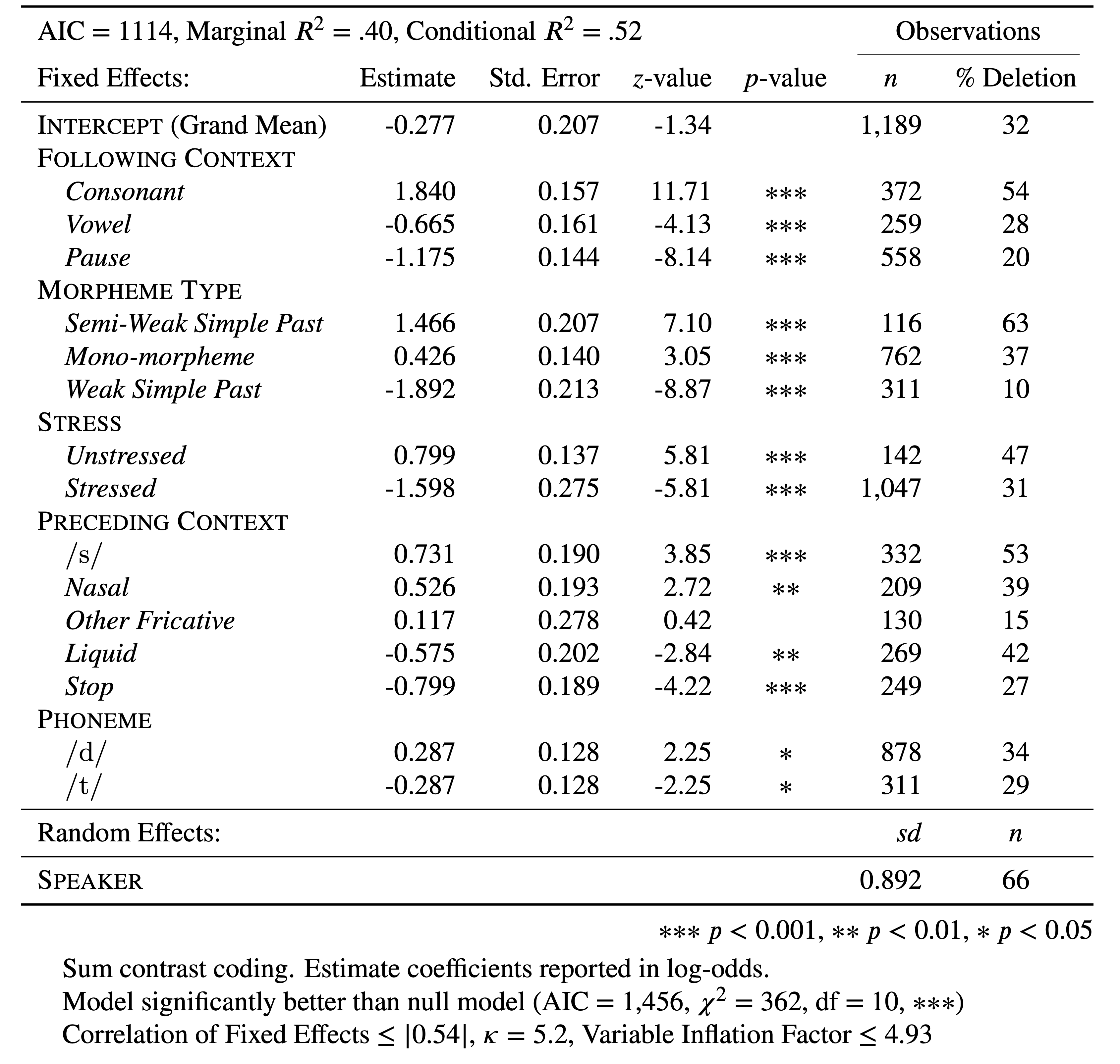
Based on the Condition Number (\(\kappa<6\)) and the VIF (\(<5\)) you can report that any (multi-) collinearity in your model is within acceptably low limits. You can add this to your manuscript table, as in Table 1 (based on td.glmer.parsimonious), though you should always contextualize what these measures indicate (i.e., low collinearity) in the text too.
Keep in mind that if there are interaction terms (e.g., Sex*Age.Group) in your model high VIF values are expected. This is because you are explicitly expecting and testing a correlation between two predictors. The (multi-) collinearity among two components of the interaction term is also called “inessential ill-conditioning”, which leads to inflated VIF values.
Also keep in mind that (multi-) collinearity might arise when a third, unobserved variable has a causal effect on two or more predictors’ effect on the dependant variable. For example, correlated Education and Job Type effects may be caused by an underlying age effect, if older speakers are generally less educated and blue-collar workers and young speakers are generally more educated and white collar workers. In such cases, the actual relationship that matters is the association between the unobserved variable and the dependant variable. If confronted with a case like this, you should revisit what independent predictors are included in the model. Non-inferential tools that can include (multi-) collinear descriptors (like Conditional Inference Trees or Random Forests) may help you.
References
Baayen, R.Harald. 2008. Analyzing linguistic data: A practical introduction to statistics using R. Cambridge: Cambridge University Press.
Belsley, David A. & Kuh, Edwin & Welsch, Roy E. 1980. Regression diagnostics: Identifying influential data and sources of collinearity. New York: Wiley.
James, Gareth & Witten, Daniela & Hastie, Trevor & Tibshirani, Robert. 2013. An introduction to statistical learning: With applications in r. New York: Springer. Retrieved from https://link.springer.com/book/10.1007/978-1-4614-7138-7c
Footnotes
Any absolute value greater than \(3\), or rather any positive value higher than \(+3\) or any negative value lower than \(-3\).↩︎
See also Notes on Interactions by Derek Denis, available at https://www.dropbox.com/s/7c4tzc8st5dmeit/Denis_2010_Notes_On_Interactions.pdf.↩︎
I checked the data and there are only three such tokens: one token of bugged and two of hugged.↩︎
Reuse
CC-BY-SA 4.0
Citation
BibTeX citation:
@online{gardner,
  author = {Gardner, Matt Hunt},
  title = {Mixed-Efects {Logistic} {Regression} {Analysis:} {Part} 3},
  series = {Linguistics Methods Hub},
  volume = {Doing LVC with R},
  date = {},
  url = {https://lingmethodshub.github.io/content/R/lvc_r/114_lvcr.html},
  doi = {10.5281/zenodo.7160718},
  langid = {en}
}
For attribution, please cite this work as:
Gardner, Matt Hunt. n.d. Mixed-Efects Logistic Regression Analysis: Part
3. Linguistics Methods Hub: Doing LVC with R. (https://lingmethodshub.github.io/content/R/lvc_r/114_lvcr.html).
doi: 10.5281/zenodo.7160718