Getting to Know Your Data

Getting a snapshot of your data. Types of data and data structures. Getting the dimensions of your data. Introducting the (t/d) dataset.

Author

Affiliation

Matt Hunt Gardner

University of Oxford

Getting to know the (t, d) deletion data

If you followed the previous section you now have an object in R called td. If not, you can load it now with either of the following codes.

td <- read.delim("https://www.dropbox.com/s/jxlfuogea3lx2pu/deletiondata.txt?dl=1")

td <- read.delim("Data/deletiondata.txt")

Getting a Snapshot of the Data

Now that you have some data loaded into R you can start exploring it. At any time you can type td into the console window to see what that object actually represents. Try it.

td

To find out how many columns there are in your data frame (this is what R calls spreadsheets), use the function nrow(). Similarly, to find out how many columns are in the data frame, use the function ncol(). The function dim() gives both.

nrow(td)

[1] 6989

ncol(td)

[1] 12

dim(td)

[1] 6989   12

There are 6,989 rows and 12 columns in this data frame.

The summary() function is one of the most useful functions you’ll use in R. It gives you a quick snapshot of a data frame.

summary(td)

   Dep.Var             Stress            Category          Morph.Type       
 Length:6989        Length:6989        Length:6989        Length:6989       
 Class :character   Class :character   Class :character   Class :character  
 Mode  :character   Mode  :character   Mode  :character   Mode  :character  
                                                                            
                                                                            
                                                                            
    Before             After             Speaker               YOB      
 Length:6989        Length:6989        Length:6989        Min.   :1915  
 Class :character   Class :character   Class :character   1st Qu.:1952  
 Mode  :character   Mode  :character   Mode  :character   Median :1965  
                                                          Mean   :1967  
                                                          3rd Qu.:1991  
                                                          Max.   :1999  
     Sex             Education             Job            Phoneme.Dep.Var   
 Length:6989        Length:6989        Length:6989        Length:6989       
 Class :character   Class :character   Class :character   Class :character  
 Mode  :character   Mode  :character   Mode  :character   Mode  :character  
                                                                            
                                                                            
                                                                            

The summary() function shows you the name of all the columns in the data frame and what each column contains.

When you import a data frame into R, R automatically decides what type of data each column contains. Any data frame columns where all cells contain only numbers are assumed to numeric or integer data (depending on if there are decimal values). Any columns that include letters will be assumed to be character data.

For numeric or integer data (like YOB, or year of birth of the speakers in the td data), the summary() function will tell you the mean, the median, the minimum value, the maximum value, and the values of the first and third quartiles. The mean is the arithmetic mean, which is the sum of all the values in a column divided by the number of values in a column. Fifty percent of the values in the column are equal to or less than the mean and 50% of the values in the column are greater than or less than the mean. The mean can also be thought of as the 2nd quartile. The median is exact middle point of the values in the column ordered from smallest to largest. For normally distributed data, the mean and the median should be close to the same value. Not all data, however, is normally distributed, which is sometimes a problem, and sometimes not a problem. If a certain test expects numerical data to be normally distributed these instructions will explain what to do, but for now, it’s just good to know what mean and median indicate. Twenty-five percent of the values in the column are equal to or less than the 1st quartile and 75% of the values in the column are equal to or less than the 3rd quartile. The minimum value is the lowest value in a column; the maximum value is the highest number in a column. These values can be used to construct a box and whisker plot:

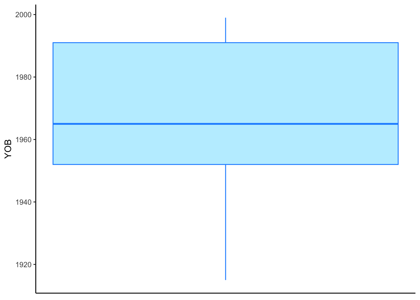
Figure 1: Box and whisker plot of YOB (Year of Birth) in the td data frame

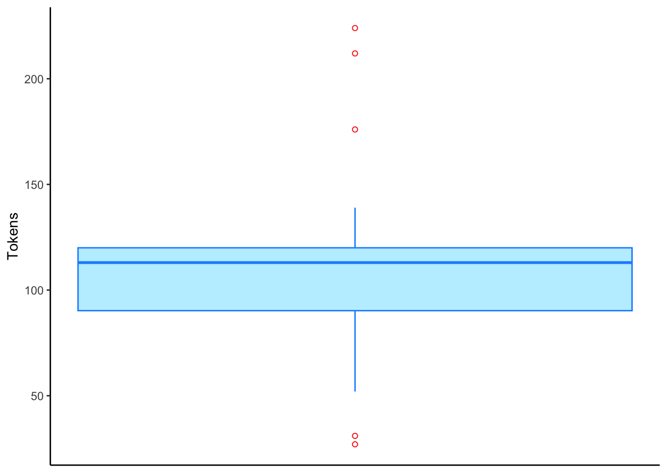
The bottom whisker ends at the minimum value of 1910. The bottom line of the box displays the first quartile value of 1952. The thick bar in the middle of the box is at the second quartile value/mean of 1965. The top line of the box ends at the third quartile value of 1991. The range from the first quartile to the third quartile is called the interquartile range. The top whisker ends at the maximum value of 1999. Sometimes extremely high or extremely low values are more than \(1.5\times\) the interquartile range from the top or bottom of the box. In these cases the whiskers will extend out to the last value within \(1.5\times\) the interquartile range and anything beyond that will be an outlier and identified with a small circle, as in Figure 2.

Figure 2: Box and whisker plot of the number of tokens per speaker in the td data frame

The function names() returns a vector (a series of items in a line, separated by commas) of the column names. This function can be useful as a quick way to get the names of each column. You will need to use these names quite often when writing other commands. colnames() returns the same information; ls() returns the same information, but ordered alphabetically.

names(td)

 [1] "Dep.Var"         "Stress"          "Category"        "Morph.Type"     
 [5] "Before"          "After"           "Speaker"         "YOB"            
 [9] "Sex"             "Education"       "Job"             "Phoneme.Dep.Var"

colnames(td)

 [1] "Dep.Var"         "Stress"          "Category"        "Morph.Type"     
 [5] "Before"          "After"           "Speaker"         "YOB"            
 [9] "Sex"             "Education"       "Job"             "Phoneme.Dep.Var"

ls(td)

 [1] "After"           "Before"          "Category"        "Dep.Var"        
 [5] "Education"       "Job"             "Morph.Type"      "Phoneme.Dep.Var"
 [9] "Sex"             "Speaker"         "Stress"          "YOB"            

The function str() describes the structure of a data frame. It reports similar information as summary() but does not include descriptions of each column; however, the layout of the information is sometimes a little easier to read, especially if your data frame has many columns. Here we can see that YOB is categorized as int (integer) data and all the other columns are chr (character) data.

str(td)

'data.frame':   6989 obs. of  12 variables:
 $ Dep.Var        : chr  "Realized" "Realized" "Realized" "Deletion" ...
 $ Stress         : chr  "Stressed" "Stressed" "Stressed" "Stressed" ...
 $ Category       : chr  "Function" "Function" "Function" "Function" ...
 $ Morph.Type     : chr  "Mono" "Mono" "Mono" "Mono" ...
 $ Before         : chr  "Vowel" "Vowel" "Vowel" "Vowel" ...
 $ After          : chr  "Pause" "Pause" "Pause" "Pause" ...
 $ Speaker        : chr  "BOUF65" "CHIF55" "CLAF52" "CLAM73" ...
 $ YOB            : int  1965 1955 1952 1973 1915 1941 1953 1953 1958 1946 ...
 $ Sex            : chr  "F" "F" "F" "M" ...
 $ Education      : chr  "Educated" "Educated" "Educated" "Not Educated" ...
 $ Job            : chr  "White" "White" "Service" "Blue" ...
 $ Phoneme.Dep.Var: chr  "t--Affricate" "t--Fricative" "t--Affricate" "t--Deletion" ...

head() will return the first six lines of the data frame. tail() provides the last six. For either you can change the number of lines reported using the option n=.

head(td)

   Dep.Var   Stress Category Morph.Type Before After Speaker  YOB Sex
1 Realized Stressed Function       Mono  Vowel Pause  BOUF65 1965   F
2 Realized Stressed Function       Mono  Vowel Pause  CHIF55 1955   F
3 Realized Stressed Function       Mono  Vowel Pause  CLAF52 1952   F
4 Deletion Stressed Function       Mono  Vowel Pause  CLAM73 1973   M
5 Realized Stressed Function       Mono  Vowel Pause  DONF15 1915   F
6 Realized Stressed Function       Mono  Vowel Pause  DONM41 1941   M
     Education     Job Phoneme.Dep.Var
1     Educated   White    t--Affricate
2     Educated   White    t--Fricative
3     Educated Service    t--Affricate
4 Not Educated    Blue     t--Deletion
5 Not Educated Service    t--Fricative
6 Not Educated    Blue    t--Fricative

The numbers on the left side of the output are the row number in the data frame.

tail(td, n = 10)

      Dep.Var   Stress Category Morph.Type Before After Speaker  YOB Sex
6980 Realized Stressed Function       Mono  Vowel Vowel  STEM42 1942   M
6981 Realized Stressed Function       Mono  Vowel Vowel  VIKF91 1991   F
6982 Realized Stressed Function       Mono  Vowel Vowel  VIKF91 1991   F
6983 Realized Stressed  Lexical       Mono  Nasal Pause  PACM94 1994   M
6984 Deletion Stressed  Lexical       Mono      S Pause  INGM84 1984   M
6985 Realized Stressed  Lexical       Mono      S Vowel  INGM84 1984   M
6986 Realized Stressed Function       Mono  Vowel Pause  GARF16 1916   F
6987 Realized Stressed  Lexical       Mono  Vowel Pause  GARF87 1987   F
6988 Deletion Stressed  Lexical       Mono  Vowel Pause  GARF87 1987   F
6989 Realized Stressed  Lexical       Mono  Vowel Pause  GARF87 1987   F
        Education     Job Phoneme.Dep.Var
6980 Not Educated Service d--Glottal Stop
6981      Student Student         d--Flap
6982      Student Student         d--Flap
6983      Student Student            d--T
6984     Educated Service     t--Deletion
6985     Educated Service t--Glottal Stop
6986 Not Educated Service    t--Fricative
6987     Educated   White            d--T
6988     Educated   White     d--Deletion
6989     Educated   White            d--D

Types of Data

There are other types of data beside numerical (like YOB in the td data) and character (like all other columns in the td data).

Types of data in R

Data Type	Description	Example
logical	either TRUE or FALSE	The answer to a question like "is x a number?", etc.
numeric	any real number, positive or negative, with or without decimal values	Vowel formant measurements, position in an audio file, household income, etc.
double	any real number, positive or negative, with or without decimal values (identical to numeric)	Vowel formant measurements, position in an audio file, household income, etc.
integer	whole numbers and their negative counterparts	year of birth, year of data collection, number of occurrences of something, etc.
complex	data that includes imaginary or unknown elements	the pythagorian theroem, i.e., \(a^2 + b^2 = c^2\), where \(a\), \(b\), and \(c\) are unknown
character	single characters (like ’F’) or strings (like "female")	gender, speaker name, etc.
raw	raw bytes	Anything expressed in bytes

Note

Character data is always enclosed in either single quotes ' ' or double quotes " ". It is common practice to use single quotes for single characters and double quotes for strings, though either type of quotation marks will work with either data type.

double is short for “double precision floating point numbers”. Don’t worry about the difference between numeric and double, because it doesn’t really matter.

It is uncommon to use raw data in sociolinguistics. Anything can be expressed in bytes. There are two functions to convert from characters to bytes, and bytes to characters. To go from characters to bytes:

raw_variable <- charToRaw("Sociolinguistics is fun")
print(raw_variable)

 [1] 53 6f 63 69 6f 6c 69 6e 67 75 69 73 74 69 63 73 20 69 73 20 66 75 6e

print(class(raw_variable))

[1] "raw"

Above the function charToRaw() converts the string "Sociolinguistics is fun" to bytes and assigns that raw data to the object raw_variable. Next the print() function displays in R the contents of the variable raw_variable. The class() function returns the type of data contained within a variable. To convert back to characters:

char_variable <- rawToChar(raw_variable)
print(char_variable)

[1] "Sociolinguistics is fun"

print(class(char_variable))

[1] "character"

Types of Data Structures

A vector and a list are the most basic types of data structures. A vector is a collection of elements, most commonly a collection of character, logical, integer, or numeric values. Values can be combined into a vector using the concatenating function c()

simple.vector <- c("Labov", "Fishman")
print(simple.vector)

[1] "Labov"   "Fishman"

We can explore the vector using some of the same functions we’ve already seen.

length(simple.vector)

[1] 2

class(simple.vector)

[1] "character"

str(simple.vector)

 chr [1:2] "Labov" "Fishman"

Lists are like vectors but can contain a mixture of different data types. Characters must be in quotation marks. Numbers in quotation marks will be categorized as characters. Numeric data is numbers without quotation marks. Integers are specificed by adding L after the number. Logical values are either TRUE or FALSE in all capital letters.

simple.list <- list("Labov", "Fishman", "2001", 1963,
    1.5, 1974L, TRUE)
print(simple.list)

[[1]]
[1] "Labov"

[[2]]
[1] "Fishman"

[[3]]
[1] "2001"

[[4]]
[1] 1963

[[5]]
[1] 1.5

[[6]]
[1] 1974

[[7]]
[1] TRUE

length(simple.list)

[1] 7

class(simple.list)

[1] "list"

str(simple.list)

List of 7
 $ : chr "Labov"
 $ : chr "Fishman"
 $ : chr "2001"
 $ : num 1963
 $ : num 1.5
 $ : int 1974
 $ : logi TRUE

You will notice that the results of the str() function show that Labov, Fishman and 2001 are all categorized as chr (character); 1963 and 1.5 are categorized as num (numeric); 1974 is categorized as int (integer); and TRUE is categorized as logi (logical).

Lists can be bigger than just one group of data. Items in a list can also be more complex than a single value.

complex.list <- list(a = "John Baugh", b = simple.vector,
    c = simple.list, d = head(td))
print(complex.list)

$a
[1] "John Baugh"

$b
[1] "Labov"   "Fishman"

$c
$c[[1]]
[1] "Labov"

$c[[2]]
[1] "Fishman"

$c[[3]]
[1] "2001"

$c[[4]]
[1] 1963

$c[[5]]
[1] 1.5

$c[[6]]
[1] 1974

$c[[7]]
[1] TRUE


$d
   Dep.Var   Stress Category Morph.Type Before After Speaker  YOB Sex
1 Realized Stressed Function       Mono  Vowel Pause  BOUF65 1965   F
2 Realized Stressed Function       Mono  Vowel Pause  CHIF55 1955   F
3 Realized Stressed Function       Mono  Vowel Pause  CLAF52 1952   F
4 Deletion Stressed Function       Mono  Vowel Pause  CLAM73 1973   M
5 Realized Stressed Function       Mono  Vowel Pause  DONF15 1915   F
6 Realized Stressed Function       Mono  Vowel Pause  DONM41 1941   M
     Education     Job Phoneme.Dep.Var
1     Educated   White    t--Affricate
2     Educated   White    t--Fricative
3     Educated Service    t--Affricate
4 Not Educated    Blue     t--Deletion
5 Not Educated Service    t--Fricative
6 Not Educated    Blue    t--Fricative

str(complex.list)

List of 4
 $ a: chr "John Baugh"
 $ b: chr [1:2] "Labov" "Fishman"
 $ c:List of 7
  ..$ : chr "Labov"
  ..$ : chr "Fishman"
  ..$ : chr "2001"
  ..$ : num 1963
  ..$ : num 1.5
  ..$ : int 1974
  ..$ : logi TRUE
 $ d:'data.frame':  6 obs. of  12 variables:
  ..$ Dep.Var        : chr [1:6] "Realized" "Realized" "Realized" "Deletion" ...
  ..$ Stress         : chr [1:6] "Stressed" "Stressed" "Stressed" "Stressed" ...
  ..$ Category       : chr [1:6] "Function" "Function" "Function" "Function" ...
  ..$ Morph.Type     : chr [1:6] "Mono" "Mono" "Mono" "Mono" ...
  ..$ Before         : chr [1:6] "Vowel" "Vowel" "Vowel" "Vowel" ...
  ..$ After          : chr [1:6] "Pause" "Pause" "Pause" "Pause" ...
  ..$ Speaker        : chr [1:6] "BOUF65" "CHIF55" "CLAF52" "CLAM73" ...
  ..$ YOB            : int [1:6] 1965 1955 1952 1973 1915 1941
  ..$ Sex            : chr [1:6] "F" "F" "F" "M" ...
  ..$ Education      : chr [1:6] "Educated" "Educated" "Educated" "Not Educated" ...
  ..$ Job            : chr [1:6] "White" "White" "Service" "Blue" ...
  ..$ Phoneme.Dep.Var: chr [1:6] "t--Affricate" "t--Fricative" "t--Affricate" "t--Deletion" ...

In the list complex.list column a contains only one value: John Baugh. Column b contains our simple.vector, column c contains our simple.list, and column d includes the first six rows of the td data (which itself has columns). To access the values from columns within columns you can use multiple $ operators.

print(complex.list$a)

[1] "John Baugh"

print(complex.list$d)

   Dep.Var   Stress Category Morph.Type Before After Speaker  YOB Sex
1 Realized Stressed Function       Mono  Vowel Pause  BOUF65 1965   F
2 Realized Stressed Function       Mono  Vowel Pause  CHIF55 1955   F
3 Realized Stressed Function       Mono  Vowel Pause  CLAF52 1952   F
4 Deletion Stressed Function       Mono  Vowel Pause  CLAM73 1973   M
5 Realized Stressed Function       Mono  Vowel Pause  DONF15 1915   F
6 Realized Stressed Function       Mono  Vowel Pause  DONM41 1941   M
     Education     Job Phoneme.Dep.Var
1     Educated   White    t--Affricate
2     Educated   White    t--Fricative
3     Educated Service    t--Affricate
4 Not Educated    Blue     t--Deletion
5 Not Educated Service    t--Fricative
6 Not Educated    Blue    t--Fricative

print(complex.list$d$Job)

[1] "White"   "White"   "Service" "Blue"    "Service" "Blue"   

Generally, in LVC analysis we do not deal often with either simple vectors or lists; instead, most of our data is in a spreadsheet-like format, which in R is a data frame.

Data frames are a special type of list in which every element in the list has the same length (unlike, for example, the complex.list above). Data frames can have additional annotations, like rownames(). Some statisticians use rownames() for things like participantID, sampleID, or some other unique identifier. Most of the time (and for our purposes), rownames() are not useful given that we have multiple rows from the same speaker/interview, etc.

Factors and Comments

A factor in R is a special type of variable or data type that, in theory, has a limited number of values. Each value is called a level. Any vector or data frame column of character or integer values can be a factor. Most non-numerical data in LVC is generally thought of as a factor already, so knowing how to convert vectors or data frame columns to factors is important. For example, in the td data, the column Stress contains only two options: Stressed and Unstressed. Because this column contains letters, when we imported it into R, it was automatically categorized as character data. This is probably the best option for a column that, for example, contained the broader context of a token. For Stress, however, it is better for our purposes for R to consider the column as containing a factor with two discrete levels. Below is the code to convert Stress into a factor.

# Determine the class of the column Stress in the
# date frame td
class(td$Stress)

[1] "character"

# Convert Stress to a column to a factor
td$Stress <- factor(td$Stress)
# Verify class of Stress column
class(td$Stress)

[1] "factor"

Notice the comments in the code above. In R any line that begins with a # is not evaluated. This is called commenting out a line. We use # to include notes in our codes, or to keep code in our script file but have R ignore it. This can be useful in order to keep track of the steps you are taking in an analysis (see also this tutorial on organizing code using #)

Columns within a data frame can be specified using the $ operator So, above, we tell R to assign (using the assignment operator <-) the values of the original td$Stress column, converted into factors, back to the column td$Stress. In other words, we are replacing the original column td$Stress with a converted version of itself. Now, look how the output of the summary() function changes.

summary(td)

   Dep.Var                 Stress       Category          Morph.Type       
 Length:6989        Stressed  :6555   Length:6989        Length:6989       
 Class :character   Unstressed: 434   Class :character   Class :character  
 Mode  :character                     Mode  :character   Mode  :character  
                                                                           
                                                                           
                                                                           
    Before             After             Speaker               YOB      
 Length:6989        Length:6989        Length:6989        Min.   :1915  
 Class :character   Class :character   Class :character   1st Qu.:1952  
 Mode  :character   Mode  :character   Mode  :character   Median :1965  
                                                          Mean   :1967  
                                                          3rd Qu.:1991  
                                                          Max.   :1999  
     Sex             Education             Job            Phoneme.Dep.Var   
 Length:6989        Length:6989        Length:6989        Length:6989       
 Class :character   Class :character   Class :character   Class :character  
 Mode  :character   Mode  :character   Mode  :character   Mode  :character  
                                                                            
                                                                            
                                                                            

We get the number of observations of each level of td$Stress instead of just the number of rows (i.e. the length of the column).

To get the levels of a factor we can use the function levels() and to get the number of levels, we can use the function nlevels()

levels(td$Stress)

[1] "Stressed"   "Unstressed"

nlevels(td$Stress)

[1] 2

More Exploring

If you only want information from a single column of the data frame, you can use the operator $ to specify which column of td you want. Here the column `Sex’ is specified.

summary(td$Sex)

   Length     Class      Mode 
     6989 character character 

levels(td$Sex)

NULL

The Sex column is still categorized as character data and so summary() only return the number of rows (length) of the column and there are no levels. To get the information we want about the Sex column (i.e., how many tokens are from male speakers and how many are from women speakers) we need to convert it to a factor first. We can either convert the the column to a factor column, or we can use the as.factor() function to have R treat is as a factor in just the following code.

summary(as.factor(td$Sex))

   F    M 
3776 3213 

levels(as.factor(td$Sex))

[1] "F" "M"

The following code changes all the character class columns to factors.

# Start with a fresh import of the (t, d) data
# into R, downloading it directly
td <- read.delim("https://www.dropbox.com/s/jxlfuogea3lx2pu/deletiondata.txt?dl=1")

# or using the version saved locally in a folder
# Data in the same location as your script file
td <- read.delim("Data/deletiondata.txt")

# Now convert each character column into a factor
td$Dep.Var <- factor(td$Dep.Var)
td$Stress <- factor(td$Stress)
td$Category <- factor(td$Category)
td$Morph.Type <- factor(td$Morph.Type)
td$Before <- factor(td$Before)
td$After <- factor(td$After)
td$Speaker <- factor(td$Speaker)
td$Sex <- factor(td$Sex)
td$Education <- factor(td$Education)
td$Job <- factor(td$Job)
td$Phoneme.Dep.Var <- factor(td$Phoneme.Dep.Var)

The (t/d) Data

Let’s look at the data now that all the character columns are factors.

summary(td)

     Dep.Var            Stress         Category        Morph.Type  
 Deletion:1747   Stressed  :6555   Function: 739   Mono     :5236  
 Realized:5242   Unstressed: 434   Lexical :6250   Past     : 782  
                                                   Semi-Weak: 971  
                                                                   
                                                                   
                                                                   
                                                                   
             Before           After         Speaker          YOB       Sex     
 Liquid         : 269   Consonant: 709   GARF87 : 224   Min.   :1915   F:3776  
 Nasal          : 209   H        : 246   INGM84 : 212   1st Qu.:1952   M:3213  
 Other Fricative: 130   Pause    :5248   MARM92 : 176   Median :1965           
 S              : 332   Vowel    : 786   HANF83 : 139   Mean   :1967           
 Stop           : 249                    CHIF55 : 135   3rd Qu.:1991           
 Vowel          :5800                    GARF16 : 132   Max.   :1999           
                                         (Other):5971                          
        Education         Job           Phoneme.Dep.Var
 Educated    :3006   Blue   :1068   t--Deletion : 981  
 Not Educated:2184   Service:2895   t--Fricative: 973  
 Student     :1799   Student:1799   t--T        : 830  
                     White  :1227   d--Deletion : 766  
                                    t--Affricate: 667  
                                    d--T        : 583  
                                    (Other)     :2189  

As shown by the summary(td) results above, the first column in the (t, d) deletion data is called Dep.Var and it includes two levels: Realized and Deletion. These two levels represent the two options for each token of (t, d). The values after each level are how many rows are coded with that level. In other words, there are 1,747 rows (or tokens) of Deletion and there are 5,242 rows (or tokens) of Realized. Notice that the order of the factor levels is alphabetical. There is a column labelled Stress which indicates if the (t, d) token is in a stressed or unstressed syllable. The Category column indicates if the word in which the (t, d) token appears is a function or lexical word. Morph.Type indicates if the (t, d) occurs in a monomorpheme (like fist), a semi-weak simple past-tense verb (like dealt ) in which there is a vowel change and a (t,d) sound is added, or a weak simple past-tense verb (like walked) in which just /-ed/ is added. Before indicates the type of sound preceding the (t, d) and After indicates the sound following the (t, d). Speaker is a unique identifier for each participant in the data (only the first six are displayed, though); YOB indicates the speaker’s year of birth, Sex his or her sex¹, Education his or her education level, and Job his or her job type. Finally, Phoneme.Dep.Var indicates the canonical underlying phoneme of the (t, d) token and a more detailed coding of the dependent variable.

Footnotes

1. These were the only two sex/gender identities reported by speakers in this data.

Reuse

Citation

BibTeX citation:

@online{gardner2022,
  author = {Gardner, Matt Hunt},
  title = {Getting to {Know} {Your} {Data}},
  series = {Linguistics Methods Hub},
  volume = {Doing LVC with R},
  date = {2022-09-27},
  url = {https://lingmethodshub.github.io/content/R/lvc_r/030_lvcr.html},
  doi = {10.5281/zenodo.7160718},
  langid = {en}
}

For attribution, please cite this work as:

Gardner, Matt Hunt. 2022, September 27. Getting to Know Your Data. Linguistics Methods Hub: Doing LVC with R. (https://lingmethodshub.github.io/content/R/lvc_r/030_lvcr.html). doi: 10.5281/zenodo.7160718